Southwestern California , specifically the region extending from Point Conception through the Los Angeles and Riverside basins to San Diego and the Mexican border, is rapidly approaching an ecological state of emergency brought about by destruction of native habitats along the coast and in inland basins. Roughly 17 million people or 56% of California's total population reside in the southwestern 8% of the state. Literally hundreds of biodiversity planning and conservation initiatives are underway in this region, ranging from region-wide conservation risk assessments to landscape-level recovery planning for endangered species such as the Stephens kangaroo rat (Dipodomys stephensi), to local restoration and mitigation projects for native grasslands, riparian woodlands, and coastal wetlands. One of the most far-reaching and innovative of these, which is part of California's Natural Communities Conservation Planning (NCCP) Program, has been underway since 1990 in response to the proposed listing of the California gnatcatcher (Polioptila californica) as a federally endangered species. At that time, local municipalities, developers and public agencies joined forces to design a rational reserve network for coastal sage scrub vegetation, which is the primary habitat for the gnatcatcher. Their goal was to achieve a change in listing of the gnatcatcher from endangered to threatened status and more generally to sustain the coastal sage scrub ecosystem while permitting development of some remaining areas
NCCP began with a regional assessment by a state-appointed team of research
biologists, who used the California Gap Analysis vegetation map along with
other information to establish the regional distribution and ownership status
of remaining extensive tracts of coastal sage scrub. This provided a broad
framework for more detailed reserve design studies and assessments that are
being conducted by individual counties. IBM-ERP Collaborator Peter Stine was
directly involved in producing an ambitious plan for a coastal sage scrub
reserve system designed for three target species, the California gnatcatcher,
the Cactus wren (Campylorhynchus bruneicapillus), and the
Orange-throated whiptail lizard (Cnemidophorus hyperythrus). This plan
entailed the production of detailed vegetation maps, compilation of existing
collection data for the targeted vertebrate species, a large field sampling
effort, and use of a GIS to facilitate modeling of coastal sage scrub habitat
conservation value based on vegetation patch size, condition and connectedness
to other habitat patches. The product of this effort is a proposed reserve
system for western San Diego County comprised of core conservation areas and
interlinking corridors (Stine 1995).
Over the past decade, conservation planners have developed a number of methods
for selecting priority areas for potential nature reserves. The evolution of
approaches has proceeded from simple scoring, where sites were ranked to
iterative heuristic methods. Although these methods differ in the objectives
they emphasize and the algorithms used, they all shared the desire to select
sites in an explicit, objective, repeatable, and efficient manner. That is,
to select a reserve system that accomplishes the most protection for the least
cost (or area). While the heuristic methods follow a logic designed to
achieve efficiency, they do not guarantee an optimal solution nor can they
measure how far from optimality they are. In fact, for most classes of
location/resource allocation problems, the greedy style heuristics
often find suboptimal solutions.
After a thorough review of existing literature, we concluded that most
approaches could be subsumed within a more general framework known as the
"maximal covering location problem" (MCLP), described in the
operations research and regional science literature twenty years ago. The
MCLP can be solved optimally, that is, no better solution exists, and most
problems of the size described for reserve selection can be solved within
reasonable computer resources. In the terminology of Operations Research, a
selected site could be said to "cover" a species if suitable habitat
for the species exists at that site.
To formulate the Maximal Covering Location Model, consider the following notation:
i = index for species to be protected
j = index for areas that can be selected for the reserve system
p = the number of areas that are to be selected for the reserve system
Ni = { j | where species i is present in area j }
Z = number of species covered by the set of sites selected for the
reserve system
The formulation of the MCLP for reserve selection is:
One note of caution is in order. The MCLP does fall within the class of
problems known as n-p hard. This means that a proven bound on computational
requirements to solve a given problem instance to optimality can not be
written as a polynomial of the problem characteristics. Thus, problems may
exist that are inherently hard to solve and may require a significant amount
of computer time to solve. In simple terms, worst case examples may exist
which may not be solvable to optimality within any available computer
resources. For most practical applications, MCLP problems can be easily solved.
We solved the MCLP model for a real application using vertebrate distribution
data prepared for the Gap Analysis of southwestern California. The database
consists of lists of vertebrate species in each of 280 quadrangles that
correspond to the United States Geological Survey 7.5' topographic map sheets
covering the southwestern region of California, USA. The regional species
pool contains 333 native vertebrates, and therefore the species-site matrix
contains of 281 columns by 333 rows.
The Maximal Covering Location Problem representing the reserve design problem
was solved in a two-step process. First species by site data were read by a
program that created a Mathematical Programming System (MPS) formatted file.
The MPS file represents a specific MCLP problem. The MPS format is an industry
standard and can be read by most general purpose integer-linear programming
systems. The second stage involved the application of a special purpose
Fortran program that utilized IBM's Optimization Subroutine Library (OSL)
subroutines to set-up and solve each MCLP. Solutions on an IBM RS-6000
workstation took an average of 2.8 seconds of CPU time over the 12 solutions,
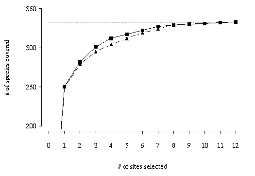
with none taking more than 9 seconds. The rate of additional species coverage
rapidly diminishes with increasing numbers of sites, such that 75% of the
vertebrate species are covered in the first site while five sites are required
to cover the last six species (Figure 12).
Figure 12. Accumulation curve showing the maximum number of new
species covered by 1 through 12 sites. The solid line with squares indicates
the curve for the MCLP model; the dashed line with triangles shows the results
of a greedy adding heuristic model.
For comparison, the tradeoff curve for a greedy adding heuristic is also shown
in Figure 12. The greedy model also selects the Catclaw Flat quadrangle in
the single site solution. Since the greedy heuristic's choice will be optimal
for the one-site solution, this selection is not surprising. However,
subsequent selections are likely to be suboptimal. Beginning with the
two-site solution, the two methods diverge as the greedy model covers fewer
species than the MCLP. This divergence in outcomes occurs because once a site
is selected in the greedy method, it remains a part of all subsequent larger
solutions. Thus, the first site selected by the greedy appears in all twelve
solutions, the site added in step 2 appears in solutions 2-11, and so on. In
steps two through seven, the greedy heuristic solution covers between three
and eight fewer species than MCLP solutions for the same number of sites. The
worst greedy solution (relative to the MCLP solution) is for the four-site
solutions, which covers 97.4% as many species. The eight- through twelve-site
solutions of both models cover the same number of species. The greedy model
took 0.63 CPU seconds.
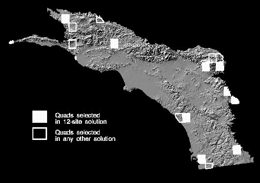
In contrast, the MCLP selects an optimal solution set for each value of p
independently of solutions for different values of p. The first site
selected does not appear in all twelve solution sets. The 12-site solution
that covers all 333 species is displayed as a map in Figure 13. Other sites
that appear in one or more of the other eleven solutions are outlined in
white. These sites generally are clustered near the sites in the 12-site
solution. Twelve sites comprises only 4% of the candidate sites in the study area.
Figure 13. Map of solution to the maximal covering location problem
in which all species are covered at least once. The twelve sites selected are
shown in cross-hatching. Sites selected in one or more of the other eleven
solutions are outlined in white.
Although the basic MCLP model proposed and applied in this report is not the
final word on reserve selection algorithms, we believe that it simplifies the
increasingly complex heuristic rule methods and gives a simple benchmark
measure of the most efficient allocation of sites. Having this benchmark
makes the trade-offs to achieve other conservation objectives and to
accommodate planning realities clear and measurable and avoids the competition
for creating the best approximation. Solution times of well under a minute
make it feasible to operate the model in an interactive spatial decision
support system. Such an interactive environment in which planners and
decision makers can explore alternatives sets based on differing objectives is
greatly needed. Furthermore, we believe that other conservation objectives
such as habitat quality, site configuration, emphasis on rare species or
additional biodiversity elements, or flexibility can all be accommodated
within the basic structure of the MCLP model, whether by additional
constraints, objectives, or weights. The MCLP approach to reserve selection
is described in greater detail in Church et al. (1996).
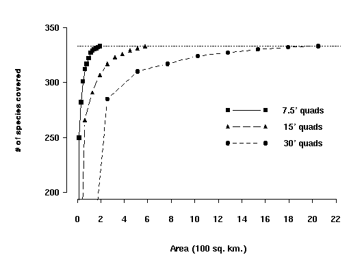
We also conducted a sensitivity analysis on the size of planning units. We
would expect larger planning units to generate less efficient solutions
because relatively few new species are accumulated as the unit grows larger.
That is, a large site would cover fewer species than four smaller sites of the
same total area if those four sites were widely distributed. In conservation
biology terms, the dispersed sites "complement" one another more
than four contiguous sites (i.e., the larger site) does. In our analysis, we
tested this hypothesis by aggregating the southwestern California vertebrate
data from units equal to the 7.5' quadrangle grid into 15' and 30' grids, each
representing a fourfold increase in area. At the 30' grid size, more than ten
times the area was required to cover all species at least once, relative to
the total area with 7.5' grids (Davis and Stoms, 1996a). The tradeoff curve
showing the relative coverage by the three grid sizes is shown in Figure 14.
Figure 14. Accumulation curve showing the maximum number of species
covered for three sizes of planning units. The line symbols for the curves
correspond to: solid line with squares = 7.5' quadrangles, the dashed lines
with triangles = 15' quadrangles, and dotted lines with circles = 30' quadrangles.
While the number of covering-type models has increased, most require custom
software or sophisticated optimization packages. Linkages with GIS have been
awkward and usually limited to data pre-processing and display of map results
or to specialized, privately distributed codes. Solving an optimal
conservation siting model has been severely limited or impossible within a
widely-used, general-purpose GIS product. Even the interactive modeling
environment described by Pressey et al. had the GIS call an external model.
To facilitate the integration of covering models into the decision making
environment, the modeling systems must be made more compatible with the
computing operations and technical skills of resource agency staff.
The MCLP model can also be reformulated as a p-median problem. This
reformulation gave us the opportunity to develop an integrated tool for
reserve selection using existing GIS software. Therefore, instead of a model
requiring external optimization software that most gap analysis projects would
not have access to and passing data back and forth with the GIS, conservation
planners could solve the problem entirely within their GIS. The application
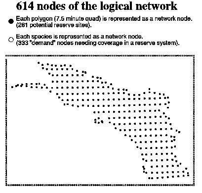
was accomplished within ARC/INFO's Location-Allocation software module. We
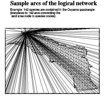
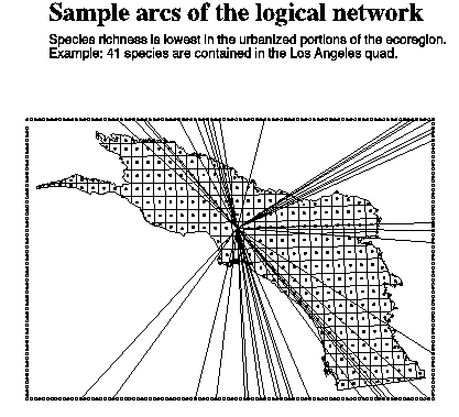
constructed a logical network structure (Figure 15) recognizable by ARC/INFO,
that translates our problem of selecting land areas to represent species into
a problem of selecting "facilities" (equivalent to reserves) that
cover "demand nodes" (equivalent to species). Finally, we extended
our approach, using the same logical network, to a weighted species coverage
model that allows us to trade-off the representation of endemic and
non-endemic species in different configurations of protected areas. The
weighted model is a move away from a simple species richness objective and
demonstrates how the MCLP (and the ARC/INFO software) can easily be extended
to optimizing more sophisticated measures of the value of a reserve system.
The approach was successfully applied to the same southwestern California data
set used by Church et al. (1996, in review) with 333 species and 281 sites.
See Gerrard et al. (in press) or
http://www.biogeog.ucsb.edu/projects/ibm/arcmodel.html
for details. More recently this approach was
extended to a national set of rare species and communities representing 3,016
elements and 5,562 sites (Chapin and Gerrard 1998).
Reserve Selection as a Maximal Covering Location Problem


